Sector Rotation with QMIT Signals
- Weichuan Deng
- Jul 9, 2024
- 13 min read
Updated: Jul 11, 2024
July 2024-- Oleg Kolesnikov, Amit Sardar & Milind Sharma
Thanks to Weichuan Deng for technical & editorial input
Executive Summary
Our objective was to test the efficacy of a sector rotation strategy based on QMIT’s flagship Sizzling Seven (Siz7) signal.
We studied two sector rotation strategies. In the first study we tested the sector rotation strategy using sector ETFs as a proxy for the sectors.
In the second study we enhanced the strategy based on ETFs by choosing the stocks with highest/lowest Siz7 ranks from the sectors that were chosen to be bought/shorted.
We tried various combinations of which Long/ Short and found that top vs bottom 2-sectors each is the best strategy in terms of hit rates & risk adjusted metrics for ETFs while 5-sectors each dominate in the single stock case which maximizes the distance between intra & inter cluster stock picks. In both phases a strategy based on single sectors [top vs bottom] has the highest concentration risk resulting in the highest volatility and max drawdowns.
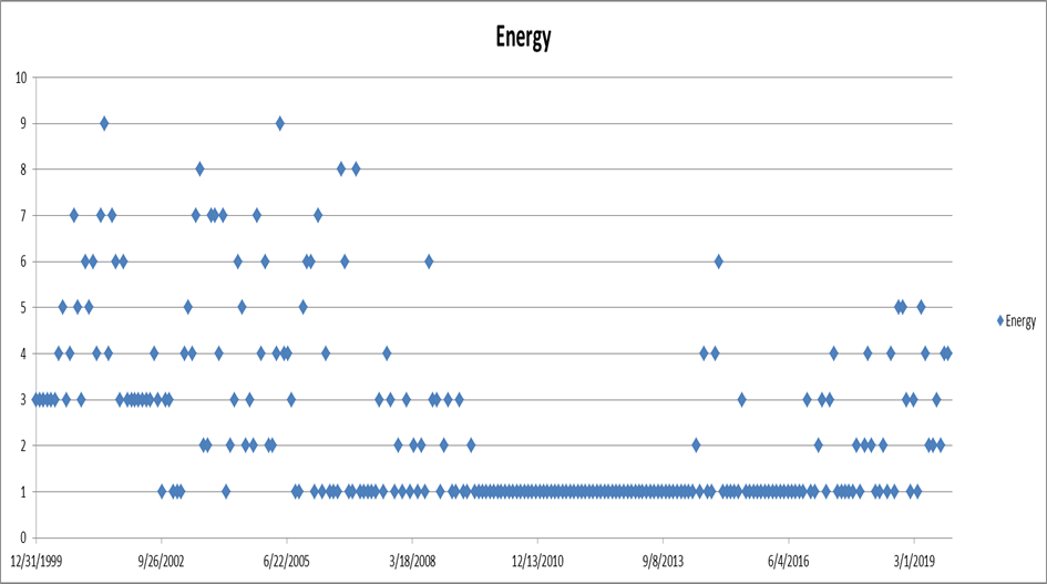
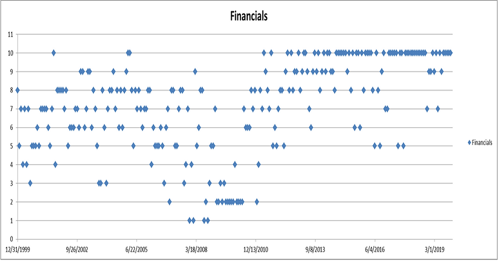
This strategy could have helped investors sit out the Financials sector during the GFC of 2008 and the Energy sector through the commodity crash of 2015 suggesting efficacy on the short side.
Why sector rotation strategies?
Sector rotation is a prominent investment strategy utilized by investors to maximize returns by timing sector exposures based on their performance outlook. This strategy capitalizes on the fact that different sectors of the economy often exhibit varying performance patterns during different phases of economic cycles, business cycles, and secular trends.
The fundamental premise behind sector rotation is that sectors will reflect the cyclicality of the respective industry groups. For example, defensive sectors like utilities and consumer staples tend to perform well during economic downturns due to their stable demand, while cyclical sectors like information technology and consumer discretionary often lead during economic expansions due to increased consumer and business spending.
Sector rotation can be implemented through various means, including exchange-traded funds (ETFs), mutual funds, or direct investments in individual stocks within targeted sectors. The effectiveness of sector rotation strategies is supported by academic research. For instance, Fabozzi, Gupta, and Markowitz (2002) provide an overview of the evolution of portfolio theory, including sector rotation strategies within the broader context of portfolio management. Moskowitz and Grinblatt (1999) examine the role of industry and sector momentum in explaining stock performance, offering insights into sector-based strategies. Fama and French (1997) explore the cost of equity across different industries, providing a basis for understanding the varying risk and return characteristics of sectors.
The diagram below shows that there’s substantial performance dispersion (as embodied by the best-worst spread) across sectors to be monetized given that sector leadership changes almost every year - driven by secular trends, business cycles, and market cycles.[1] In this white paper, we investigate whether one can utilize QMIT’s Siz7 (Sizzling Seven) bottom-up stock-based signals to generate high risk adjusted return long/ short sector level strategies. The application of bottom-up stock-based signals in investment strategies also has been well studied. Piotroski (2000) discusses the effectiveness of fundamental analysis in identifying high book-to-market firms and their subsequent performance.

Figure 1: Annually Sector Returns
QMIT’s Factor library and Enhanced Smart Betas
A factor is a security attribute which has been identified as a potential driver of return or risk. Hence, in a multi-factor model, companies in the estimation universe are ranked on each of these factors (or evaluation metrics), and then in conjunction via some function of these factors. Factor investing is therefore the embodiment of an investment strategy in which securities are chosen based on certain desirable characteristics with the goal of increasing exposure to those factors or to improve overall risk adjusted long-term returns.
While factor ranks are developed based on a single definition, QMIT’s Enhanced Smart Betas (ESBs) on the other hand, combine a range of factors within each cohort with the objective of outperforming the naïve benchmark factor. Smart Betas which therefore represent thematic clusters of factors like Value or Growth are often also called interchangeably called Risk-Premia in industry parlance, although a-priori one need not expect all Smart Betas to deliver Risk-Premia. The Smart Beta label started as a marketing gimmick and has caught on to the extent that it allows for the differentiation of “smarter” fundamental factor-weighted indices vs the default market cap weighted ones.
QMIT has developed 18 different ESBs based on extensive factor research over the past 21 years. To prevent look-ahead bias in representing a single 21+ year time series for a given ESB, QMIT uses a BFOM trading strategy which picks the “Best Flavor of the Month” based on cumulative LTD return through T-1, ex ante, which pre-empts look ahead bias. Finally, QMIT then constructs a series of composite signals based on these ESB BFOMs which we deploy towards testing our sector rotation strategy.
Below is an overview of all QMIT ESBs and composite signals:

As mentioned earlier, ESBs combine a range of factors within each cohort with the objective of outperforming the naïve benchmark factor. Below is the graph of cumulative returns for QMIT’s Deep Value (DV) vs the Fama-French Book-to-price (its benchmark factor).
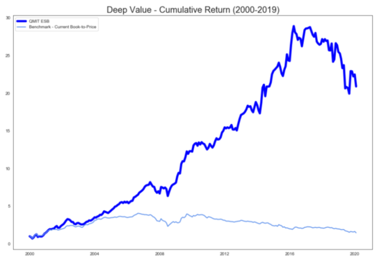
Figure 2: Cumulative Return of Deep Value vs. Fama-French Book-to-price - 20Y
In fact, almost all QMIT ESBs outperform their corresponding benchmarks in terms of Beta-Neutral Sharpe and Sortino Ratios.
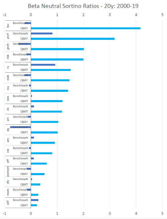
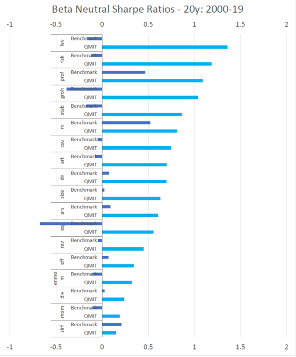
Figure 3: BFOM Beta-Neutral Sharpe ratios - 20Y Figure 4: BFOM Beta-Neutral Sortino ratios – 20Y
QMIT’s Sizzling Seven signal
For this white paper, we focus on deploying the Sizzling Seven MFM alpha signal, which is QMIT’s proprietary combination of ESBs meant to demonstrate the merits of combining QMIT’s high octane ESBs towards formulating turnkey signals for hedge funds.
QMIT’s Sizzling Seven composite multi-factor model includes:
Quality Composite
Quality – Leverage (LEV) - Captures excess returns to stocks with low leverage.
Quality – Profitability (PROF) - Captures excess returns to highly profitable stocks.
Quality – Capital Structure/ Usage (CSU) - Captures excess returns to firms with better usage of capital.
Quality – Stability (STAB) - Captures excess returns to stocks with stable financial ratios.
Quality – Efficiency (EFF) - Captures excess returns to stocks that are characterized by high operating efficiency.
Quality – Earnings Quality (EQ) - Captures excess returns to stocks that are characterized by low accruals.
Value Composite
Deep Value (DV) - Captures excess returns to value stocks based on intrinsic value metrics.
Relative Value (RV) - Captures excess returns to value stocks based on relative valuation metrics.
Growth + Momentum Composite
Analyst Revisions (ARS) - Captures excess returns of stocks with momentum on account of analyst revisions.
Analyst Ratings (ART) - Captures excess returns to stocks that track analyst recommendation and target.
Enhanced Momentum (EnMoM) - Captures excess returns to stocks experiencing trend continuation.
Growth (GroH) - Captures excess returns to stocks that have higher-than-average historical growth.
Risk (RISK) - Captures excess returns to stocks with lower-than-average volatility, beta, and/ or idiosyncratic risk.
Size (SIZE) - Captures excess returns to smaller firms.
Reversals (REV) - Captures excess returns to stocks with lackluster past performance that is due for a rebound.
Short Interest (SIRF) - Captures excess returns to stocks with lower Short Inter.
Methodology
Sector Choice
The first step is aggregating bottom-up single stock ranks to determine the descending rank order of sectors which would then yield the top vs bottom sectors for back-testing the spread returns based on ETFs as sector proxies. We use QMIT’s Siz7 month end (single stock level) signal ranks to determine the descending rank order of sectors. QMIT’s signal data includes monthly factor scores from [0 – 100] for ~2500 tickers from 12/31/1999 to 12/31/2019. We make the prediction in the following steps:
We labelled each ticker based on QMIT’s sector labelling, which includes Utilities, Energy, Communication Services, Consumer Discretionary, Financials, Consumer Staples, Information Technology, Materials, Industrials, and Health Care.
QMIT’s sector labelling is based on a mapping table maintained by the firm using Factset industry codes.[2]
For every month, we will calculate a sector signal score based on the average rank for stocks labelled in that sector. We exclude real-estate because it is not as suitable in a generic quant model. We then rank the 10 sectors from 1-10 based on signal strength.
We now have a prediction each month as to which sector is going to perform best/ worst in the next month.
Phase 1 – Strategy based on single ETFs
The simplest way to reflect bullish or bearish views on a sector is to utilize liquid, institutionally tradable sector ETFs. For each of the 11 sectors, SPDR provides a corresponding sector ETF (e.g., XLF, XLU) that one can use.[3] Subsequent to the exclusion of Real Estate, we then obtain the adjusted prices to compute monthly total returns for the remaining 10 sectors. We implement the strategy by going long the sectors with the highest scores and shorting the sectors with the lowest scores. Below, we present the back-test results of long/short cases ranging from 1 to 5 sectors in each direction with a starting capital of $100 Million as the AUM. We have the following assumptions:
Gross exposure of 200% = GMV = 100% LMV + 100% SMV with and Net MV = 0% at each rebalancing month end date.
Month-end rebalancing on e.g., formation date 03/31/00 ranks would be utilized for monetizing the strategy returns in the calendar month of April 2000.[4]
Each sector is equally weighted at the time of rebalancing based on the cum VAMI. We present results of long/short 1 to 5 sectors in each direction.[5]
Result highlights
Picking fewer sectors consistently yields higher returns given the more concentrated bets, which suggests predictive efficacy of the underlying Siz7 signal. Given that higher signal scores are supposed to imply higher predicted stock returns, implementing this at the aggregated sector level should yield similar results. This hypothesis is confirmed by the results presented herein.
However, picking 1 sector each yields much higher annual volatility and drawdown than picking 2 sectors at a time. The 2-sector strategy appears to be the optimal choice with the highest hit rate, Sharpe and Sortino ratio due to significantly reduced drawdowns from the 1-sector strategy[6] per below. This shows the benefits of diversification.
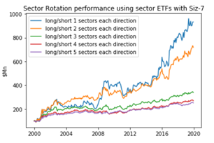
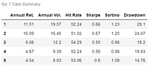
Figure 5: Sector Rotation Performance Using Sector ETFs with Siz-7
Phase 2 - Strategy based on single stocks
Signal construction
In Sector Choice, we got a prediction each month as to which sector(s) is/ are going to perform best/ worst in the next month. In Phase 2, we now chose the best/ worst stocks within each sector rather than just using Sector ETFs as a proxy.
We choose the stocks based on their Siz7 ranks and whether the sector is a buy or a short.
The number of stocks we invest in is normalized by adjusting to the number of sectors invested in. This is done to make the performance results comparable between strategies using different number of sector
Implementing the strategy
We implement the strategy by going long the sectors with the highest scores and shorting the sectors with the lowest scores. Within the best sectors we go long the best stocks with highest siz7 ranks (in the top decile or quintile) and analogously we must short the worst stocks (bottom decile or quintile) in the worst sectors while ensuring a minimum of 35 stocks on each side. However, given the varying sector sizes, the total number of top decile or quintile names picked on each side may differ subject to the minimum. For the case of 5x5 sectors, if the intra-sector number of stocks is less than 7 then we must ensure a minimum of 7 stocks with equal weights to satisfy the minimum of 35 names.
Below, we present the back-test results of long/ short cases ranging from 1 to 5 sectors in each direction with a starting capital of $100 million. We have the same assumptions as Phase 1 with additional following assumption - viz., that all stocks are also equally weighted within each sector (where the sectors themselves are equally weighted on each side).
Results
Picking more sectors consistently yields higher returns and lower volatility with risk adjusted outcomes.
Picking 1x1 sector results in much higher volatility and drawdowns than picking 2 or more sectors at a time. This shows the benefits of diversification.
Comparing the top decile vs top quintile scenarios, we see that performance metrics and returns are better for the top decile case. Given the 5.33 Sortino for the top decile with 5x5 sectors it’s clear that’s the winning strategy. Thus, we see that our sector rotation implemented with single stocks provides much better risk adjusted performance by virtue of maximizing the intra & inter cluster distances of scores.
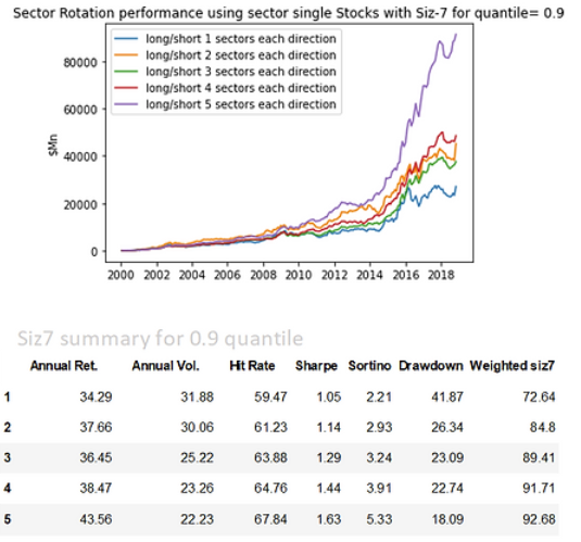
Figure 6: Sector Rotation Performance Using Single Stocks (top vs bottom 10%) with Siz-7
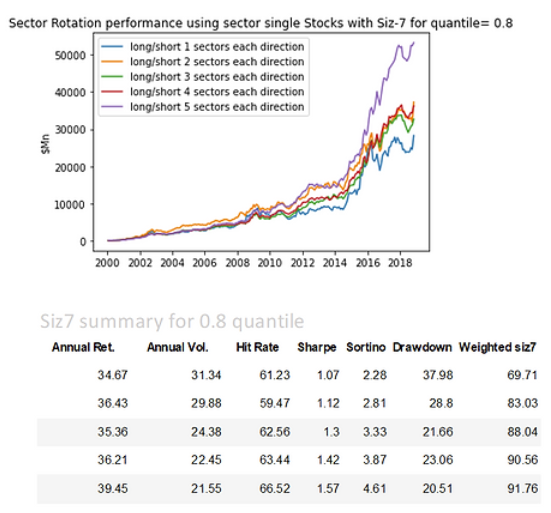
Figure 7: Sector Rotation Performance Using Single Stocks (top vs bottom 20%) with Siz-7
Comparison of Phase 1 and Phase 2
We see that the strategy based on single stocks results in risk-adjusted performance that is higher than the one based on ETFs by a multiple. In Phase 1, the best risk adjusted performer was the 2-sector case with a Sharpe ratio of 0.67. In Phase 2, the best risk adjusted performer for choosing top vs bottom 20% and 10% stocks was the 5 not 2 sector case with a Sharpe of 1.57 and 1.63 respectively. Thus, we see that our sector rotation implemented with single stocks provides much better risk adjusted performance by virtue of maximizing the intra & inter cluster distances of scores. Given the 5.33 Sortino for the 90% quantile with 5x5 sectors it’s clear that’s the winning strategy since it is not only better than other single stock cases but also 4.9x better risk adjusted than the 1.09 Sortino for the best ETF case. This is because in the ETF scenarios the returns decay in tandem with the volatility despite greater diversification across more sectors resulting in not much of a risk adjusted gradient whereas in Phase 2, we see the best of both worlds. Not only do the returns increase significantly as we monetize the top-ranked stocks across multiple sectors but with lower strategy volatility due to greater diversification across more sectors.
Regressions
For each signal, we would like to assess how well it explains returns. To do so, we performed the following steps:
Since we are trying to capture relative returns, we normalized the sector returns each month by the mean of the 10 sector returns.
Similarly, we also normalized the 10 sector scores each month.
For each month, we have 10 x-y pairs. We pooled 240 months together and now we have 2400 x-y pairs, with x as a sector score, and y as next month’s sector return.
With these data points, we then performed an OLS regression, and observed:
There is clear statistical significance in Siz7 ranks predicting relative sector returns in the following month.
The IC (information coefficient) is highly significant in the quantitative finance context.
R-square | 0.049 |
t-stat | 10.786 |
Correlation | 0.221 |
Table 1: Regression Result
Top sector picks
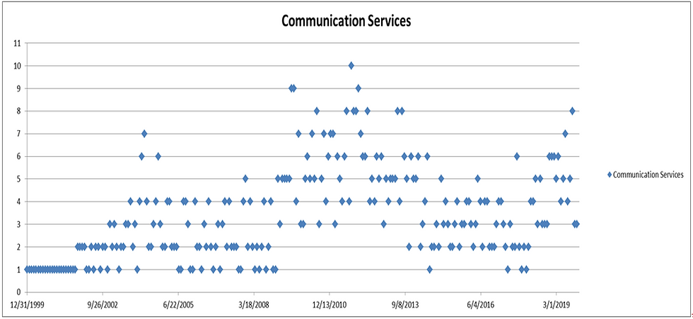
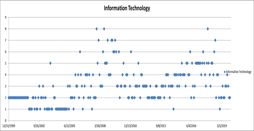
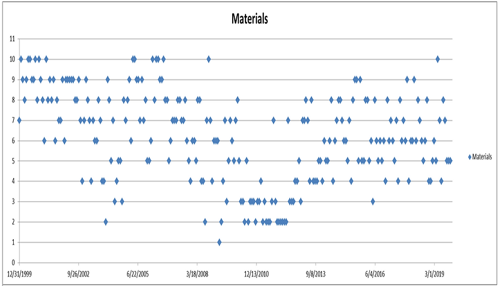
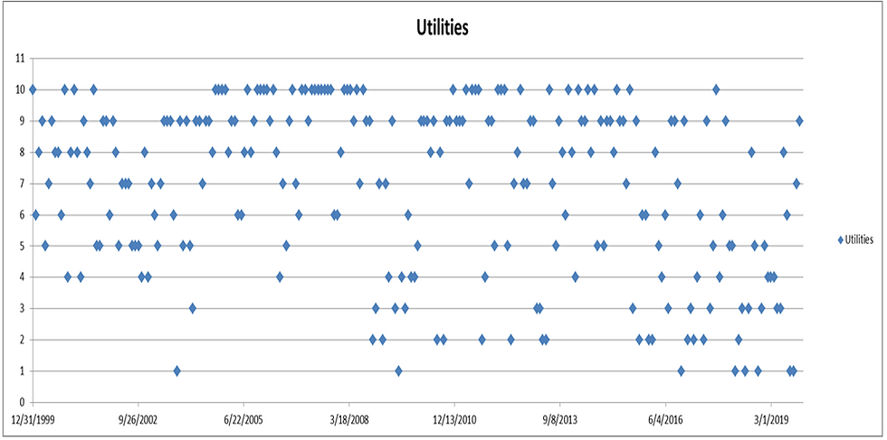
Below, we show for each sector the percentage of times that it receives a certain score in the past 20 years. For instance, Communication Services has a score of 1 (worst sector) for 19.6% of the months in the past 20 years for Sizzling Seven. In below, we also show dot plots of time series scores for each sector which leads to the following observations:
The sector that is most frequently held long happens to be Consumer Staples followed by Utilities, due to consistently high Siz7 scores on average over time. The preference for most defensive sectors may be a reflection of the success of low volatility investing as well as a function of the two crashes in the 20y dataset.
Financials were rarely shorted except around the GFC.
The most frequently shorted sector is Energy reflecting poor Siz7 scores on average over time. Looking at the plot, we observe that the strategies shorted energy consistently before and after the commodity crash of 2015. On the other hand, Industrials, Staples & Discretionary are rarely at the bottom of the sector ranks.
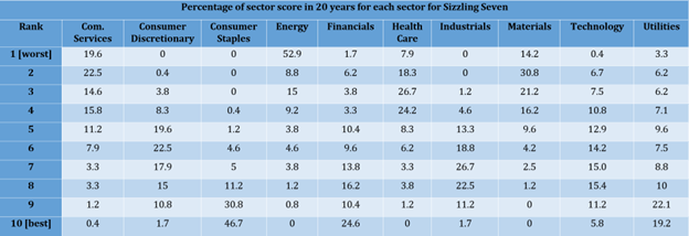
Figure 7: Percentage of Sector Score in 20 years for each Sector for Sizzling Seven
Sizzling Seven Sector Ranks
Aggregate sector ranks are the same whether one implements the strategy based on ETFs or single stocks.



Conclusions
QMIT’s Sizzling Seven MFM signal clearly has some predictive content in being able to sort sector winners vs. sector losers over the past 19 years.
For case of investing in single ETFs, picking 2 sectors top vs bottom yields slightly lower returns in comparison to picking just the best vs worst sector, but the diversification benefits dramatically outweigh the return trade off given the much lower volatility and max drawdowns.
For case of investing in single stocks, picking the top 5 vs bottom 5 sectors yields slightly higher returns in comparison to picking just the best vs worst sector. Moreover, we also get the diversification benefits.
Using top/bottom 10% stocks within the sectors yields better performance results than using 20%. Overall, volatility is a bit higher which shows benefits of diversification but these benefits are not that high. To conclude, there is no significant difference in performance results for the top 10% vs 20% cases but based on risk adjusted metrics we should take 0.9 quantile (top 10% of stocks) for 5x5 sectors.
Our final implementation of the rotation strategy uses single stocks within the sectors which substantially outperforms the case using ETFs in both risk-adjusted and nominal performance.
References
[1] E. Fama and K. French, "Common Risk Factors in the Returns on Stock and Bonds," Journal of Financial Economics, vol. 33, 1993.
[2] J. Green, J. R. Hand and X. F. Zhang, "The characteristics that provide independent information about average u.s. monthly stock returns," Review of Financial Studies, vol. 30, no. 12, pp. 4389- 4436, 2017.
[3] N. Jegadeesh and S. Titman, "Returns to Buying Winners and Selling Losers: Implications for Stock Market Efficiency," The Journal of Finance, vol. 48, no. 1, pp. 65-91, 1993.
[4] D. Ung and S. Abburu, “Sector Rotation: Can the Approach Work in Different Countries?”, State Street Global Advisors SPDR, 2021
[5] F. J. Fabozzi, F. Gupta and H. M. Markowitz, "The Legacy of Modern Portfolio Theory," Journal of Investing, vol. 11, no. 3, pp. 7-22, 2002.
[6] T. J. Moskowitz and M. Grinblatt, "Do Industries Explain Momentum?" Journal of Finance, vol. 54, no. 4, pp. 1249-1290, 1999.
[7] E. F. Fama and K. R. French, "Industry Costs of Equity," Journal of Financial Economics, vol. 43, no. 2, pp. 153-193, 1997.
[8] J. D. Piotroski, "Value Investing: The Use of Historical Financial Statement Information to Separate Winners from Losers," Journal of Accounting Research, vol. 38, pp. 1-41, 2000.
Footnote
[1] Based on SPDR Sector Select ETF. For Communication Services, where there is insufficient data, we use the Communication Services Select Sector Index as a tradable proxy.
[2] We exclude some tickers that we cannot find the right labelling, which accounts for less than 1% of total date-ticker combinations. Each data has no more than 2% of missing tickers, and most dates have 0-1% of missing tickers.
[3] SPDR: A Standard & Poor's Depositary Receipt, or SPDR, is a type of exchange traded fund that began trading on the American Stock Exchange (AMEX) in 1993 when State Street Global Advisors' investment management group first issued shares of the SPDR 500 Trust (SPY). XLF: The Financial Select Sector SPDR® Fund; XLU: The Utilities Select Sector SPDR® Fund, are example of some of the ETF we used. We removed Real Estate because of its insufficient data, and it is unsuitable in a generic quant framework. For the SPDR communication sector ETF, it has a short history due to a change of GICS classification system in 2018, but the underlying index has 20+ years of data. Hence, we use the underly index, which is the Communication Services Select Sector Index instead as our proxy.
[4] To be careful one would take the 03/30/00 rank file available pre-open on 03/31/00 order to enter the trade at the close of 03/31/00; not that the sector ranks would be likely change in that single day.
[5] For instance, long/short 1 sector means that for every month end, we rebalance the portfolio to 100% weight long the highest score sector, and 100% weight short the lowest score sector. Choosing 5 sectors means that we long the top 5 sectors with 20% weight each, and short the bottom 5 sectors with 20% weight each.
[6] We define hit rate here as the percentage of months that the strategy yields positive returns, which necessarily means that the long sectors outperform the short sectors.
DISCLAIMERS: This white paper is not intended for trading purposes. QMIT does not recommend making investment decisions without appropriate due diligence on the part of the investor. QMIT does not provide any form of advice (investment, tax, legal) amounting to investment advice, or make any recommendations regarding particular financial instruments, investments or products. Further, QMIT reserves the right to discontinue or alter the contents of this white paper at any time, without notice. QMIT does not guarantee or warrant the accuracy, completeness or timeliness of the White Paper. For more detailed disclaimer, please refer to: QMIT disclaimers


Comments